
MetaboLabPy
Basic 2D-NMR Data Processing
2D-Jres Data Processing
To read in the 2D-Jres NMR dataset, we use the 2D-Jres example script in the script tab, as indicated below. The phrase ‘Replace with directory containing Bruker data’ should be replaced by ‘interactive’. data_sets = [] needs to be replaced by data_sets = [1, 2, 3, 4], which is also indicated in the figure below.
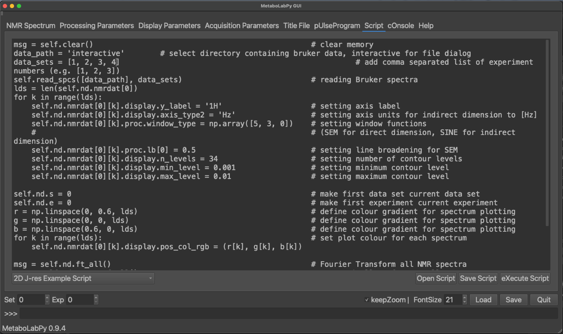
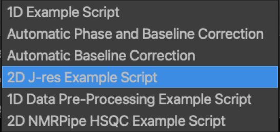
The script can then be executed either by clicking on eXecute Script in the bottom right hand corner, or via the keyboard shortcut Ctrl + x (or ⌘ + x on macOS). Please select the folder containing the directories 1, 2, 3 and 4. The program window should look like the following:
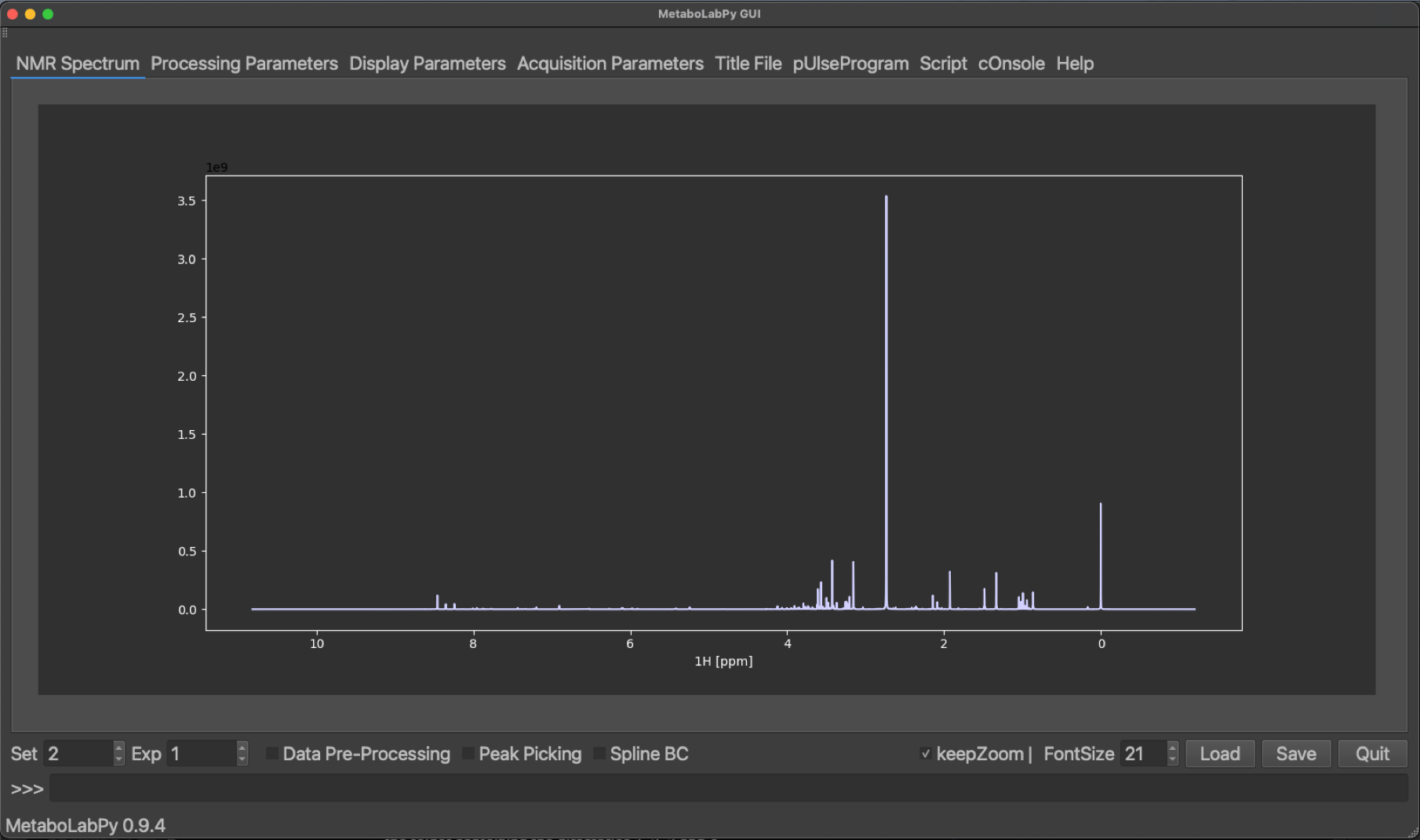
Please note, despite reading in a 2D-NMR spectrum, a 1D-NMR spectrum is displayed. This is a 1D-projection of the 2D-Jres spectrum, which is performed as part of the data processing script. Please refer to the comments in the script for details.
In order to see, the corresponding 2D-Jres spectrum, we need to change the dataset number from 2 to 1.
Processing options for 2D-NMR spectra are very similar to those for 1D-NMR data. The biggest difference is, that we have an independent set of NMR data processing parameters for every dimension. To demonstrate the effect of some processing parameters specific to 2D-Jres NMR spectra (Tilt and Symmetrize). The standard setting for these parameters is Yes for both. The Tilt option changes the spectrum, so that different components of a spectral multiplet are collapsed to the same resonance position. Symmetrize then helps to remove some 2D-Jres specific spectral artefacts.
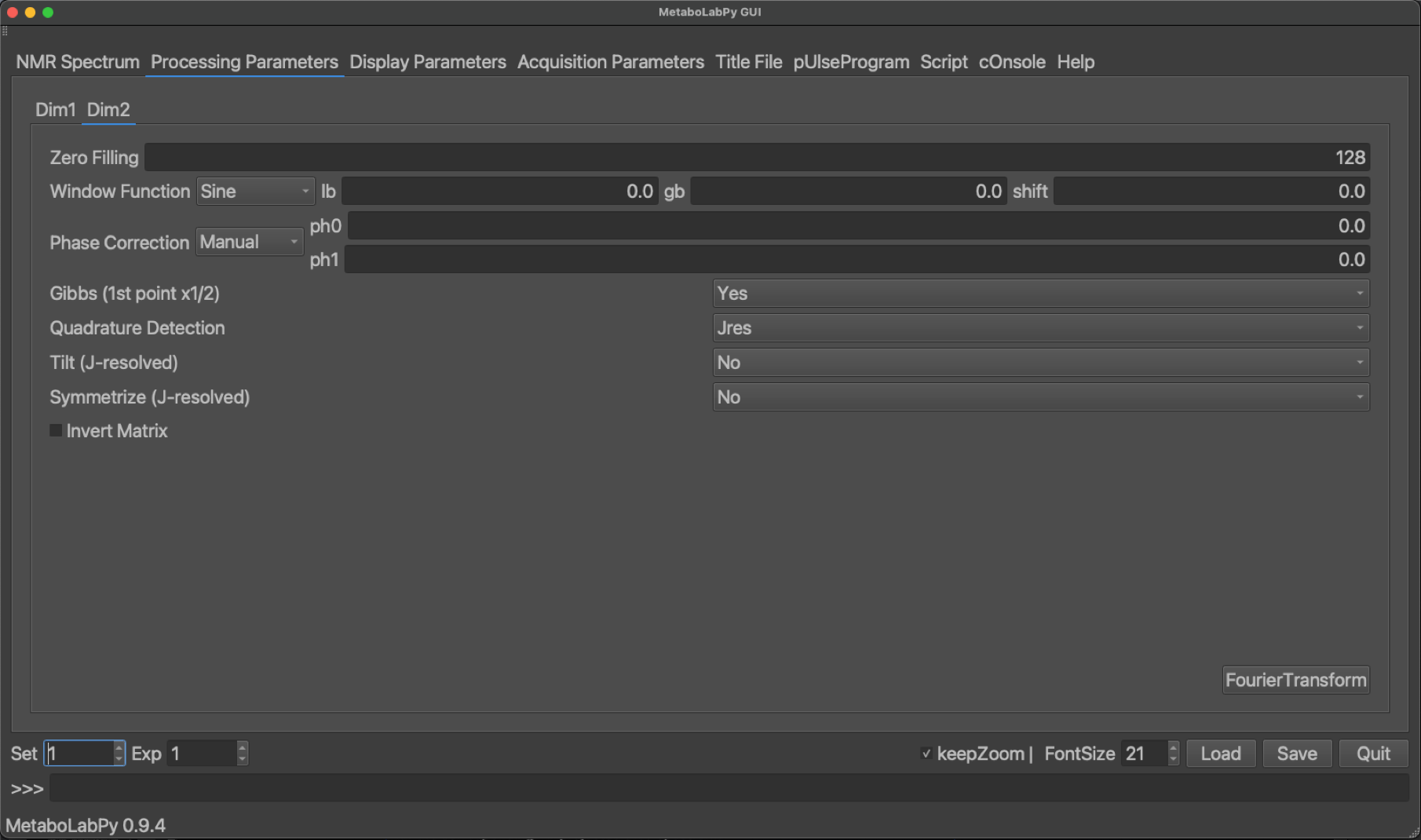
A spectrum, which was processed with both options set to No is shown below together with the corresponding 1D-projected Jres spectrum.
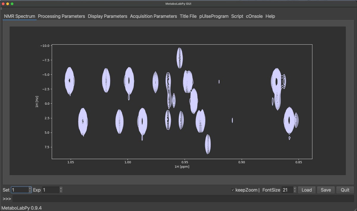
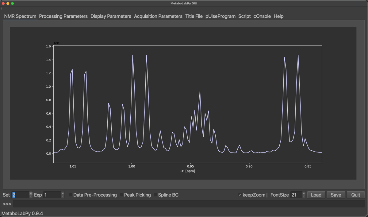
We find, that the projected Jres spectrum looks very similar to a basic 1D-1H NMR spectrum. However, once we turn the two options back on, get the following result.
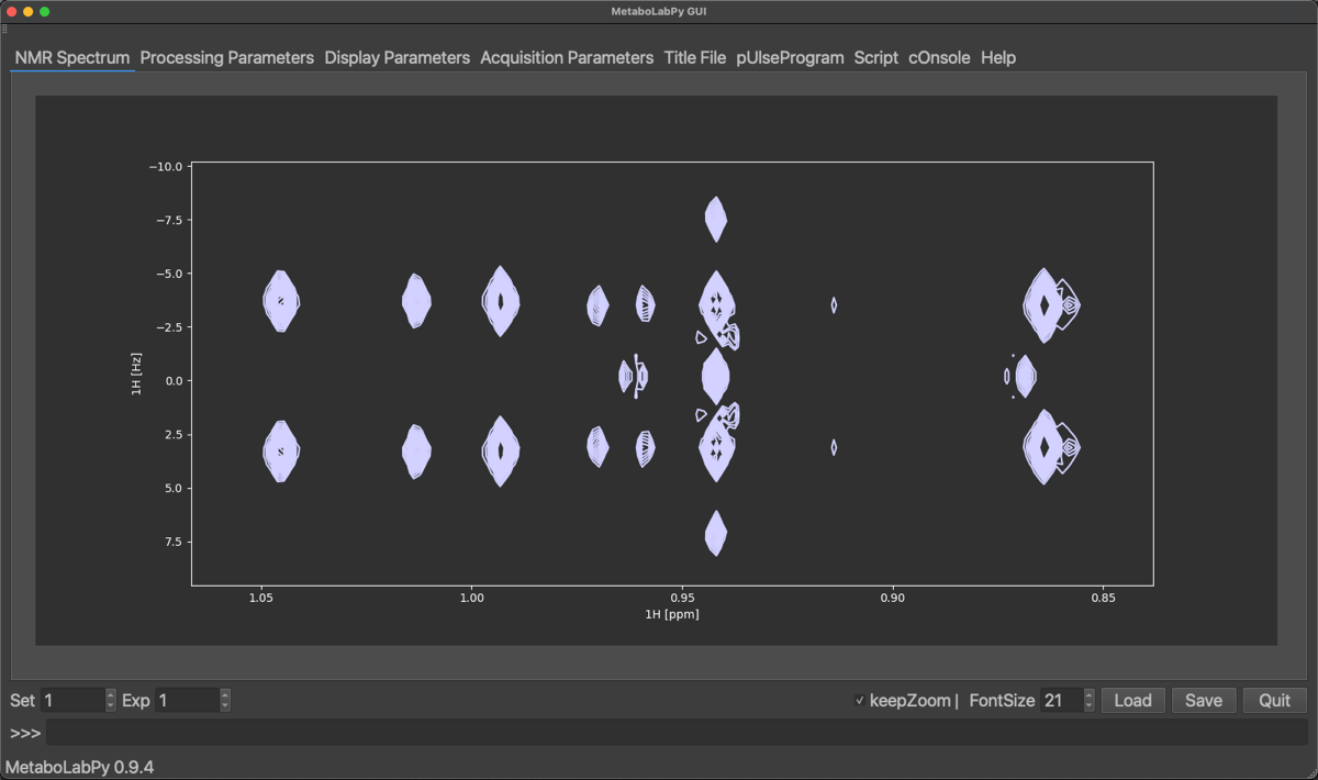
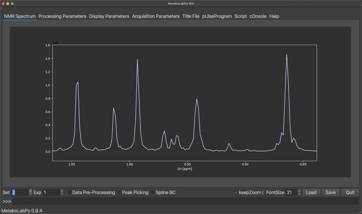
The result of using these processing options is, that the projected 1D-NMR spectrum basically looks like a proton-decoupled 1D-1H NMR spectrum. This can be useful if spectral congestion is a problem. Please also note, that the data pre-processing option is available for projected Jres spectra, so that projected Jres spectra can be prepared for multivariate data analysis in the same way as normal 1D-1H NMR spectra.
Because 2D-Jres NMR spectra are magnitude spectra, there is no need for a two-dimensional phase correction. Therefore, we will look into 2D-phase correction using phase-sensitive 2D-1H,13C HSQC NMR spectra.
The 2D-HSQC NMR dataset can be downloaded here. This dataset contains two 2D-1H,13C HSQC NMR spectra. The first dataset was acquired using conventional sampling and can be Fourier transformed within MetaboLabPy. This dataset can be opened by clicking “Open NMR Spectrum” in the File menu or by using the keyboard shortcut Ctrl + o (⌘ + o on macOS). Please select the folder number 1 to read in the spectrum. The resulting spectrum display should look similar to this:
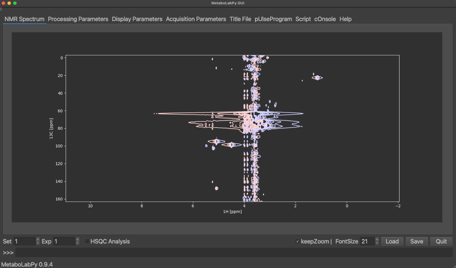
The red contour lines correspond to negative values in the 2D-NMR spectrum and the blue contour lines to positive parts of the 2D-NMR spectrum. To phase correct this 2D-NMR spectrum, we need to enter phase correction mode by clicking on Phase/Baseline Correction and then on Interactive Phase Correction in the Data menu. This will add six buttons to the GUI.

In order to perform a 2D-phase correction, we need to pick at least 2 peaks. One of the peaks should be at the right hand side of the visible signals and another peak on the left-hand side. To select a peak, click on Pick Row/Col and then click the horizontal centre of a peak. We can zoom in and out to easily select the centre of the peaks. The selected peaks are displayed a coloured crosses as demonstrated below:
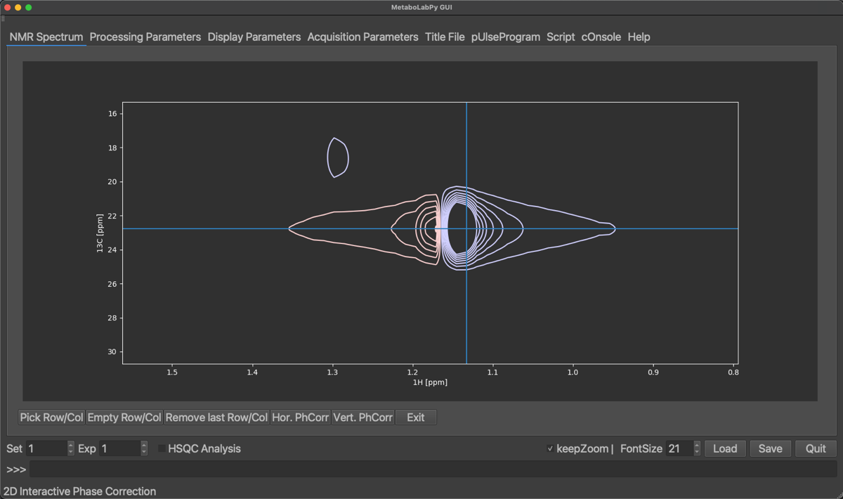
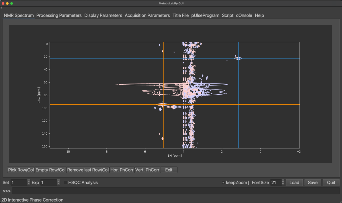
Selected peaks can be removed by clicking on Empty Row/Col (this will remove all selected peaks) or by clicking on Remove last Row/Col, which will remove only the peak selected last. Once enough peaks have been selected, we can start with the horizontal phase correction by clicking on Hor. PhCorr. The spectrum display will then display the selected rows of the spectrum with colours indicating, which peak was selected. The plotted spectra also display the pivot, which if it was not set previously, will be in the middle of the spectrum. As for 1D phase correction, it can be moved by dragging the middle mouse button over to either the right-most or left-most peaks. If there is no 3-button mouse available Ctrl + left mouse button (⌘ + left mouse button on macOS) can be used instead. The horizontal dimension can then be phase corrected by dragging the left (zero order) or right (first order, ⇧ + left mouse button) mouse button until all peaks are phase corrected.
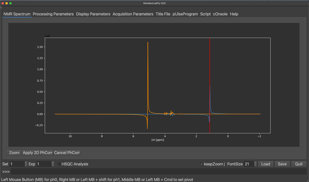
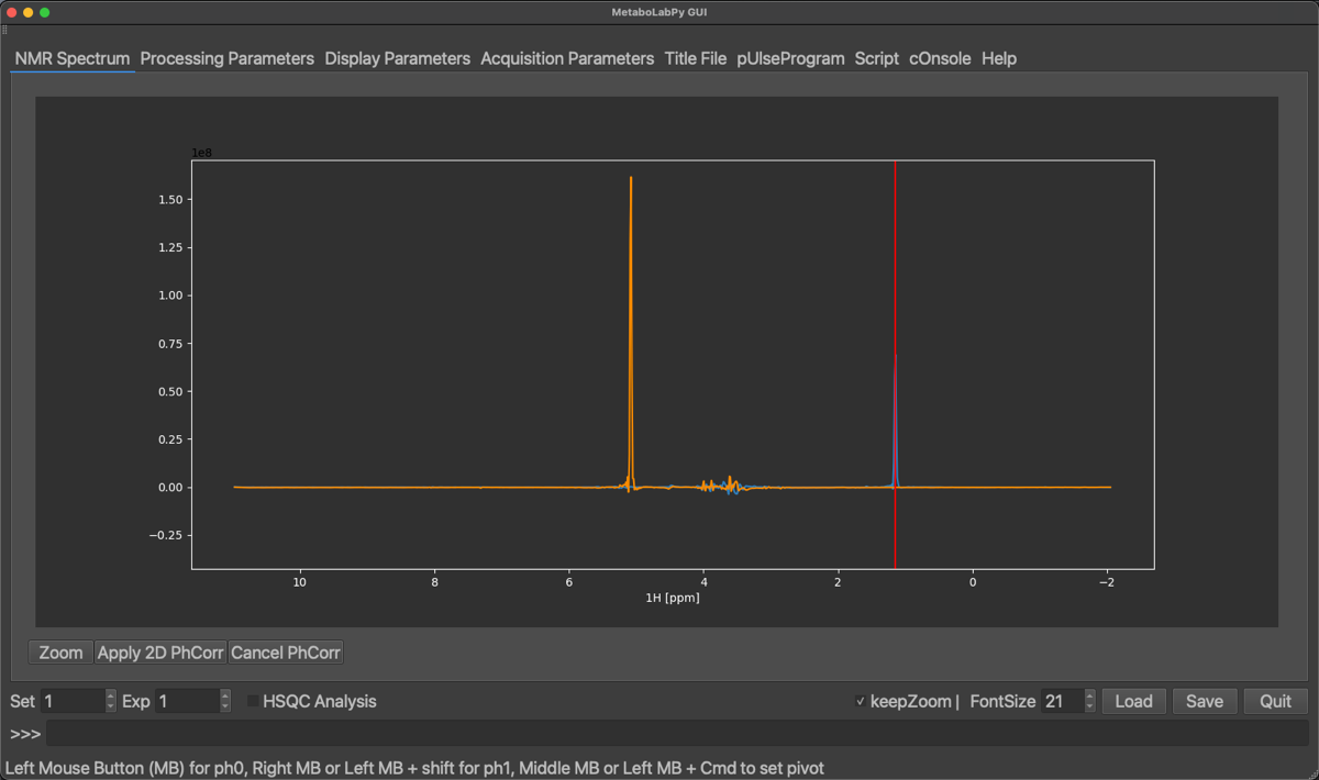
Once all peaks are phase corrected in this 1D display, the 2D-NMR spectrum can be horizontally phase corrected by clicking on Apply 2D PhCorr, alternatively the procedure can be cancelled. The 2D-NMR spectrum will be displayed again.
To phase correct the vertical dimension, remove all previously selected peaks by clicking Empty Row/Col and select a peak on top and one from the lower end of the 2D-NMR spectrum. Use zoom to ensure to select the centre of the peaks.
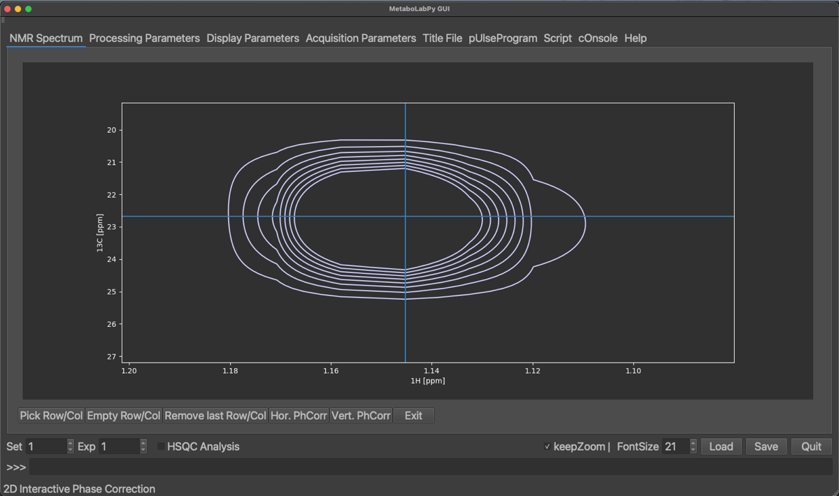
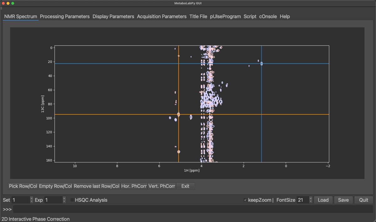
Now select Vert. PhCorr and repeat the procedure as for horizontal phase correction. After applying the vertical phase correction, phase correction mode can be exited by clicking on Exit.
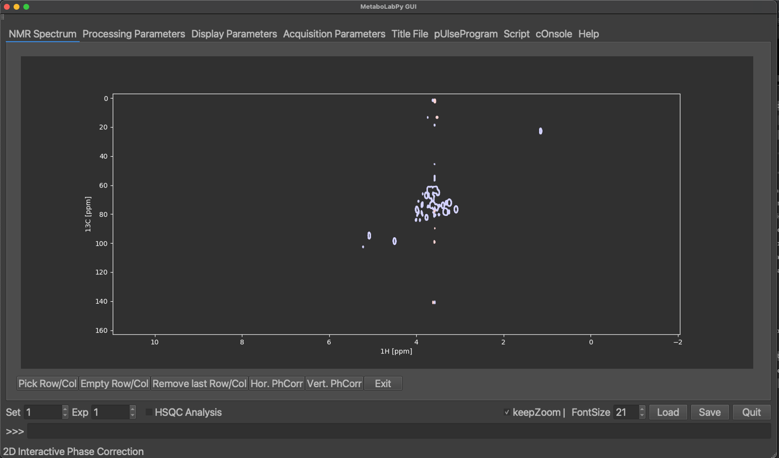
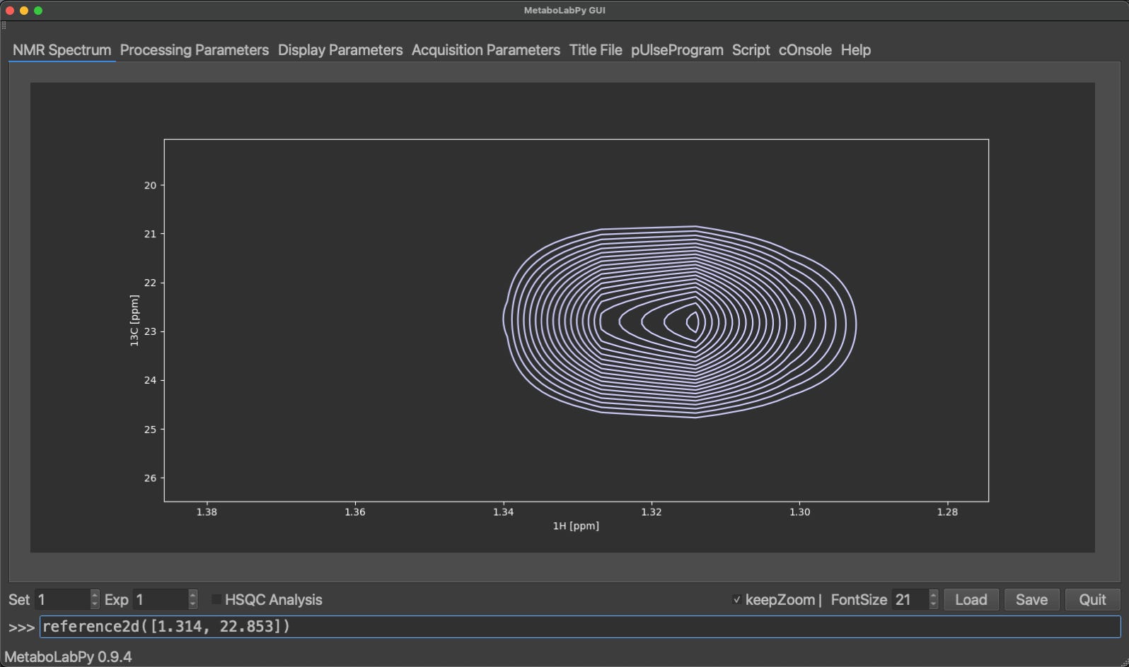
To reference 2D-NMR spectrum, zoom in to the signal to be used for referencing. Depending on the signal, there are two ways to reference the 2D spectrum. If you know the spectral coordinates, you can reference the spectrum by typing reference2d([1H chemical shift, 13C chemical shift])and then clicking the centre of the peak, or if the metabolite causing the peak signal is known, typing reference2d(‘L-LacticAcid’, 2) and clicking the centre of the peak. ‘L-LacticAcid’ is an example, because the signal selected is the methyl group signal of lactate. There will be further examples in Tracing Analysis in MetaboLabPy.
If NMR spectra were processed with the help of the excellent NMRPipe software, processed 2D-NMR spectra can be read in by clicking on Open NMRPipe in the File menu or by using the keyboard shortcut Ctrl + n (⌘ + n in macOS).
In order to successfully read in a NMRPipe processed NMR spectrum, the data needs to be organised in a specific way. If NMRPipe in conjunction with MDDNMR is used to reconstruct 2D-NMR spectra from non-uniformly sampled NMR data, the structure already exists. The original Bruker data folder containing the originally acquired spectrum (e.g. 2) needs to be in the same folder as the directory containing the processed data (e.g. 2.proc). Please note that both folder names start with the same number, but the folder containing the processed spectrum adds .proc to that.
After clicking Open NMRPipe, you will be presented with a GUI file selected. Navigate to the folder containing the processed spectrum and select the spectrum file (test.dat in our example dataset), all acquisition data will then be read from the Bruker data folder together with the processed 2D spectrum. The spectrum can be phase corrected and referenced in the same way a conventionally processed 2D-NMR spectrum can be phase corrected and referenced.
Lastly, quite often highly-resolved 2D-1H,13C HSQC NMR spectra benefit from baseline correction. This can be performed automatically using a polynomial baseline correction, by typing autobaseline2d() at the MetaboLabPy command line.