MetaboLabPy
Basic 1D-NMR Data Processing
To demonstrate basic 1D NMR data processing in MetaboLabPy, we are using two metabolite standard NMR datasets available at the BMRB NMR database (https://bmrb.io/metabolomics/). The metabolites we are going to use for this demonstration are L-Lactate and L-Glutamate.
We load the NMR data into MetaboLabPy by clicking on “Open NMR Spectrum” in the file menu or by using the keyboard shortcut Ctrl + O in windows or ⌘ + O in macOS to load in the data for L-Lactate and then repeat the same procedure to read in the data for L-Glutamate. In order to plot each spectrum in a different colour, we select the Display Parameters tab and select a colour for each of the spectra.
There are a few steps as part of every basic NMR data processing protocol. This includes the following steps:
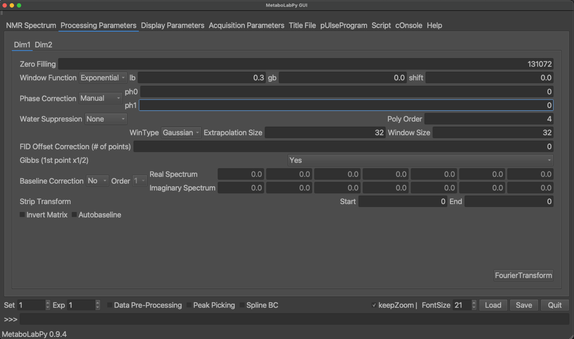
To enter into the interactive phase correction mode, we click on Phase/Baseline Correction and then on Interactive Phase Correction in the Data menu. Alternatively, we can also use the keyboard shortcut Alt + p (⌥ + p). However, before we enter into interactive phase correction mode, we select the first NMR spectrum as phaseReference experiment in the Display Parameters tab of the first NMR spectrum.
When the interactive phase correction mode is active, the status line on the bottom of the main window changes and indicates mouse actions to perform an interactive phase correction on the current spectrum. In addition to the spectrum, a red line appears, which indicates the position of the pivot, i.e. the position in the NMR spectrum at which first order phase correction has no effect. Please also note that in order to zoom in and out of the spectrum, we need to click on zoom to switch into zoom mode. Once we adjusted the view, we need to exit zoom mode to return to the phase correction mode.

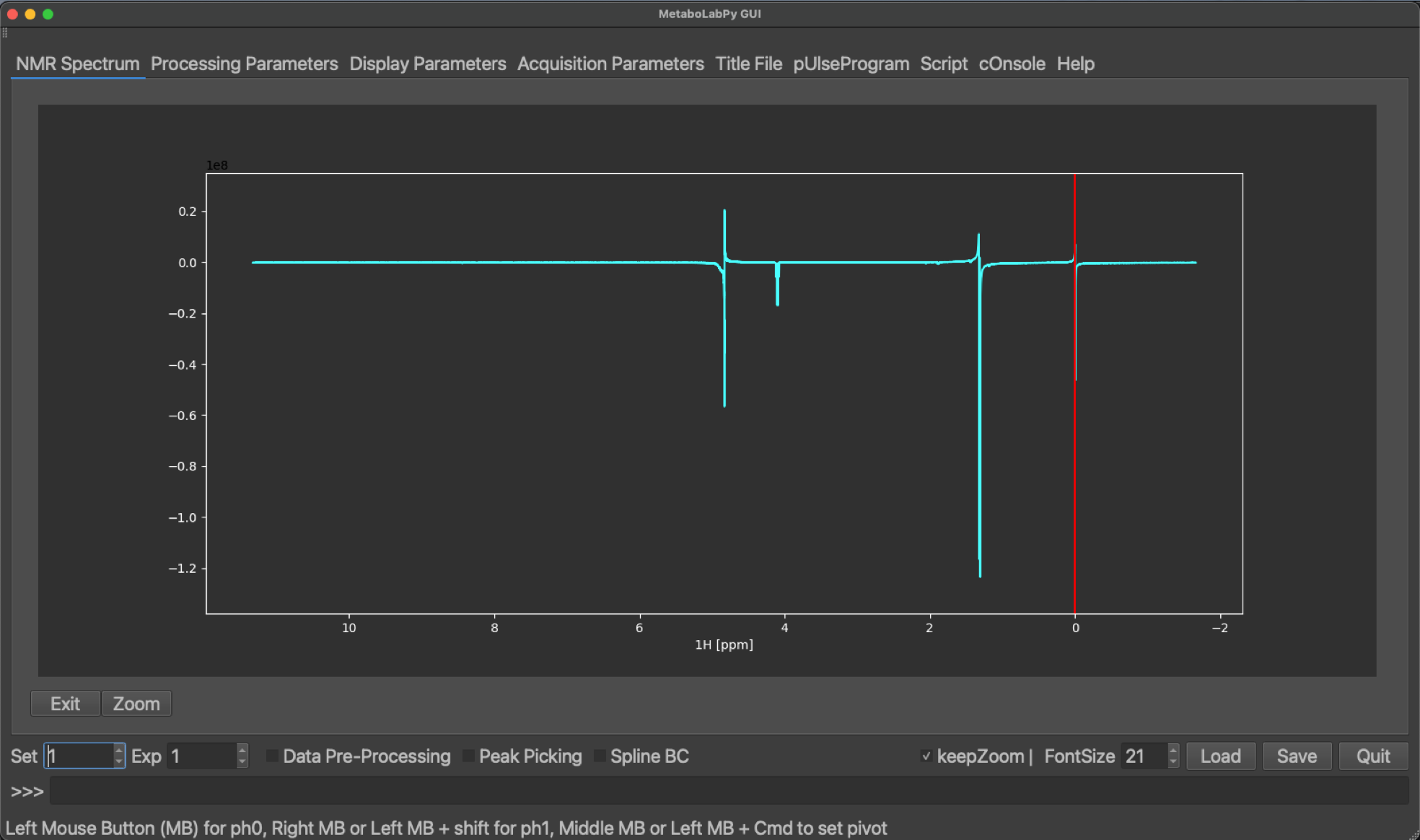
To enter into the interactive phase correction mode, we click on Phase/Baseline Correction and then on Interactive Phase Correction in the Data menu. Alternatively, we can also use the keyboard shortcut Alt + p (⌥ + p). When the interactive phase correction mode is active, the status line on the bottom of the main window changes and indicates mouse actions to perform an interactive phase correction on the current spectrum. In addition to the spectrum, a red line appears, which indicates the position of the pivot, i.e. the position in the NMR spectrum at which first order phase correction has no effect. Please also note that in order to zoom in and out of the spectrum, we need to click on zoom to switch into zoom mode. Once we adjusted the view, we need to exit zoom mode to return to the phase correction mode.
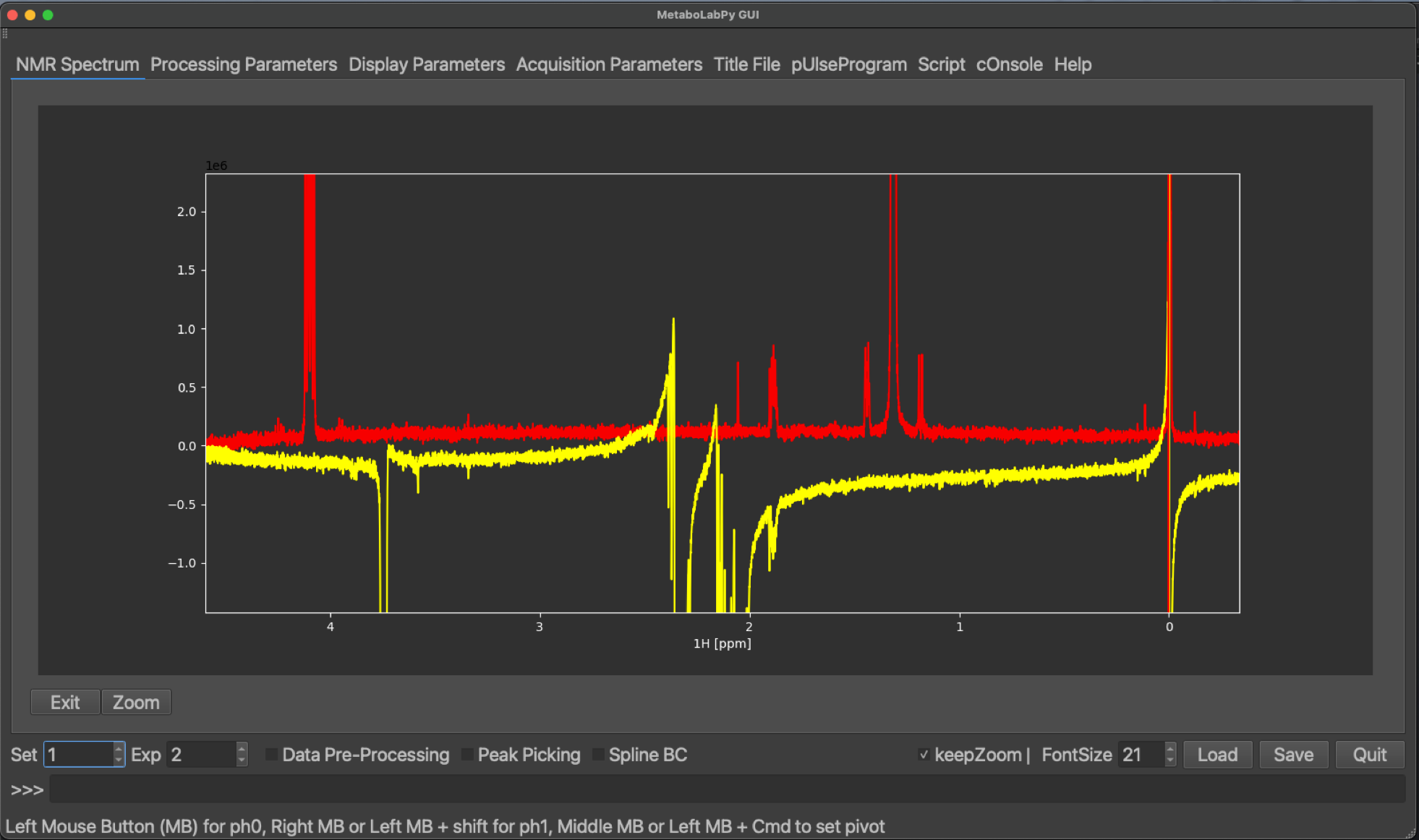
Once the first NMR spectrum is sufficiently phase corrected, we can change to the next NMR spectrum but either clicking the up-arrow in the Exp counter, enter the number 2 into the text field followed by pressing enter, or by using the keyboard shortcut Alt + cursor key up (⌥ +
Once the last spectrum has been phase corrected, interactive phase correction mode can be left by clicking on Exit or through the keyboard shortcut Alt + p (⌥ + p).
A video showing another interactive demonstration of basic 1D NMR data processing in MetaboLabPy can be found below:
After the NMR spectra have been phase corrected, automated baseline correction can be used to correct the spectral baseline. MetaboLabPy uses the pybaselines package, documentation can be found here:
In order to prepare a set of 1D NMR spectra for statistical data analysis, several steps have to be performed. MetaboLabPy provides GUI elements to facilitate this process, which is also known as data pre-processing. The data pre-processing GUI is made available by clicking on the “Data Pre-Processing” checkbox. Data to follow this tutorial can be downloaded here.
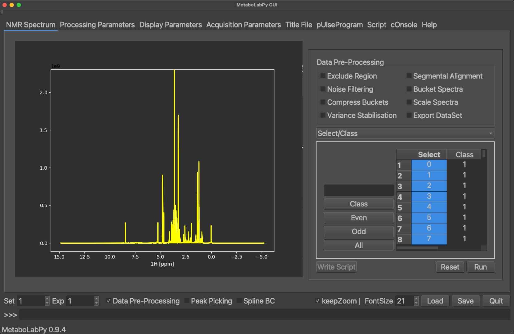
In the following paragraphs we will systematically go through all different steps of NMR data pre-processing in the order they are performed during data pre-processing.
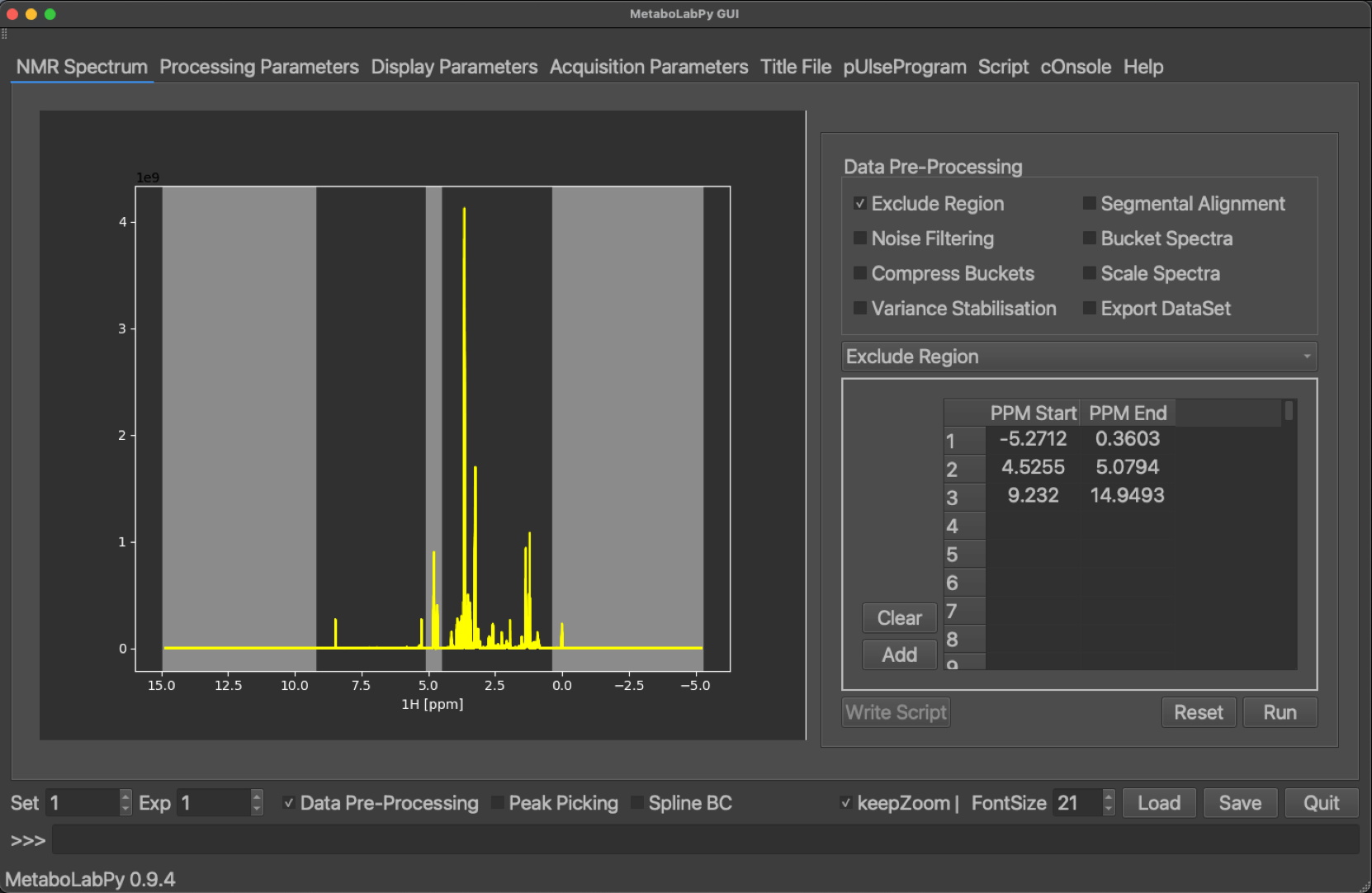
Normally 1D NMR spectra for metabolomics studies are acquired with a few ppm worthwhile of empty spectrum at the edges of the NMR spectrum. This is done deliberately to achieve a flat baseline in all peak-containing regions of the spectrum. Because those areas of the NMR spectra do not contain any signals and only noise, this spectral noise can negatively impact statistical data analysis. Therefore, these regions are excluded from analysis. Because most metabolomics samples are in aqueous environments, the middle of the spectrum is usually centred on the water signal. This signal is suppressed. However, there will still be a residual water signal left and therefore this spectral region is excluded from the analysis as well. Finally, we need to exclude the TMSP signal, because we are only interested in differences of endogenous metabolites. Because the TMSP signal is usually the rightmost signal in these NMR spectra, the exclusion area on the right-hand side of the spectrum is usually extended to include the TMSP signal.
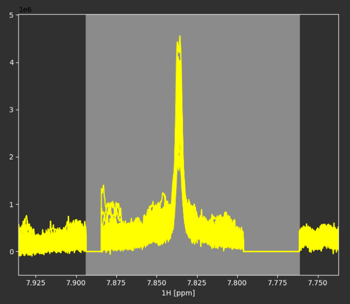
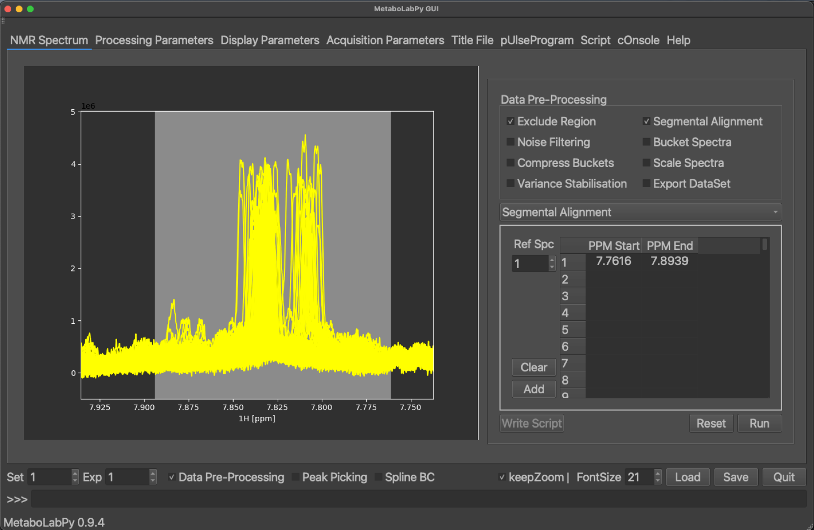
Because different samples may have small differences in their pH values, we may find some areas in the NMR spectra where NMR peaks move from sample to sample. To facilitate statistical analysis, we can align those areas independent of the rest of the NMR spectra through segmental alignment.
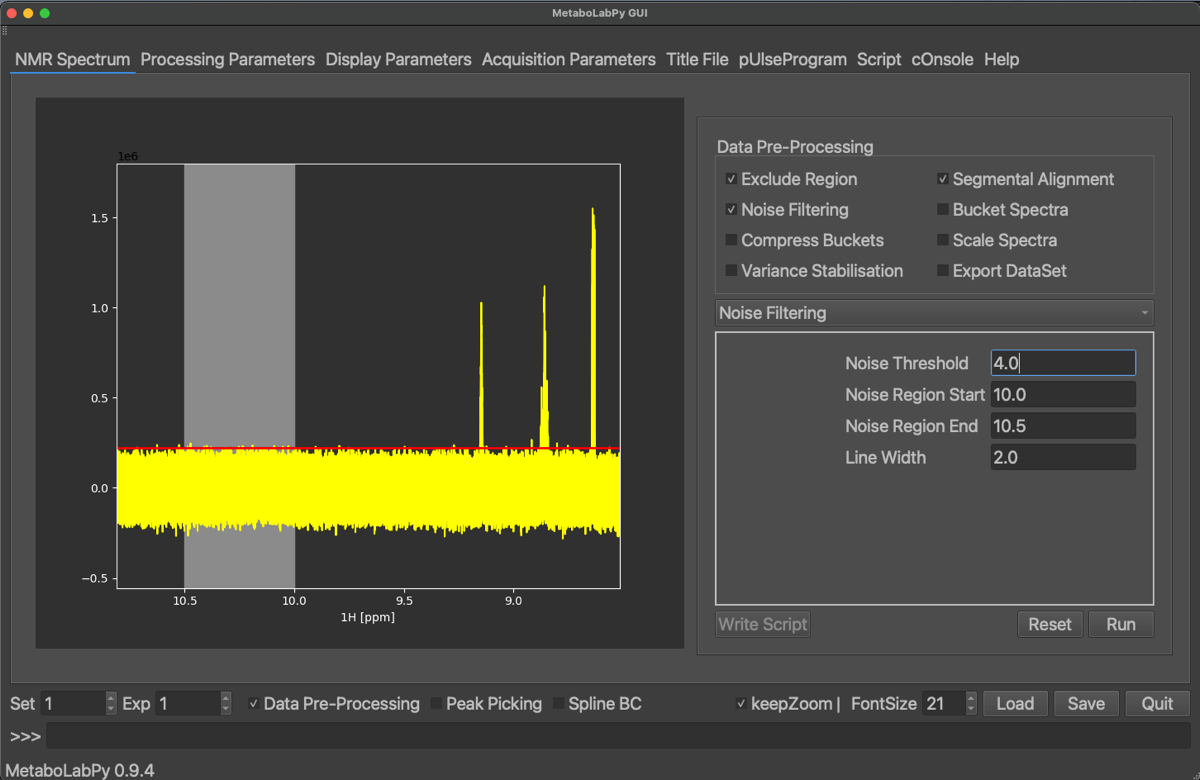
Furthermore, any area in the NMR spectra below a certain noise threshold can be removed from the data matrix to minimise noise. NMR spectra are then bucketed so that each individual data point represents a width of 0.005 ppm. After that, especially for urine and blood samples, it is important to scale the different NMR spectra to minimise effects from different sample dilutions. This is usually achieved using probabilistic quotient normalisation.
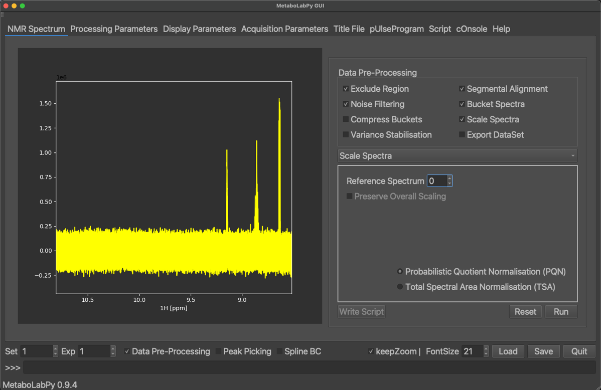
The final step of data pre-processing, before export to a useful data format, is then variance stabilisation, which is usually achieved using Pareto scaling of the data. The exact data format for export depends which platform should then be used for statistical data analysis. The Phenome Centre Birmingham (PCB) uses an Excel spreadsheet format, which e.g. MetaboAnalyst uses a csv-based format. Please have a look at the video to see a practical demonstration of all these steps.