MetaboLabPy
Scripts & Jupyter Notebooks
While most everyday data analysis options can be easily set and executed via the MetaboLabPy GUI, at least partially automated tasks can make data analysis quicker and more reproducible. Reading in a series of 1D-NMR spectra is such an example. While we could click the Open NMR Spectrum for each spectrum separately, this procedure is not very efficient. Because MetaboLabPy is built as a set of python classes, computational actions can be easily scripted in MetaboLabPy. The Script tab in the GUI is a good example for this. To facilitate standard actions such as reading in NMR spectra or setting processing parameters, a set of example scripts is included in MetaboLabPy. Each example script is well documented using comments at the end of each code line. In addition we can use non-GUI MetaboLabPy classes and methods via a Jupyter-notebook. There is a series of example Jupyter notebooks distributed with the metabolabpy package.
In the following we will look at two specific examples, highlighting small differences when using the scripting interface from within the MetaboLabPy GUI and when using Jupyter notebooks.
Let’s start with a script to read in a series of 1D-1H NMR data. Please download an example 1D-NMR dataset here. Locate the example scripts pop-up menu located on the lower left corner of the Script tab. Click on ‘1D Example Script’. This will load the text for the 1D example script. Now, change ‘Replace with directory containing Bruker data’ with ‘interactive’ and replace the square brackets in the line below with the expression np.linspace(1, 4, 4, dtype=int). This creates a numpy array with the numbers 1, 2, 3 & 4. Alternatively we could have specified each dataset number explicitly and replaced [] with [1, 2, 3, 4]. After these modifications, we should have a script like this:
msg = self.clear()
data_path = 'interactive' # select directory containing bruker data, interactive for file dialog
data_sets = np.linspace(1, 4, 4, dtyp=int) # add comma separated list of experiment numbers
self.read_spcs([data_path],data_sets) # reading Bruker spectra
msg = self.nd.set_zero_fill([131072]) # zero fill to 131072 data points
msg = self.nd.set_lb([0.3]) # 0.3 Hz line broadening
msg = self.nd.set_window_type([1]) # exponential window function
msg = self.nd.ft_all() # Fourier Transform all NMR spectra
msg = self.nd.auto_ref_all() # automatically reference to TMSP
self.nd.e = 0 # make first spectrum the current experiment
self.set_ph_ref_exp(1) # select reference spectrum for manual phase correction
After script execution (either clicking eXecute Script or via the keyboard shortcut Ctrl + x on Windows or ⌘ + x on macOS) the four spectra in that dataset should have been read in, all FIDs will be exponentially line broadened by 0.3 Hz, zero-filled to 131072 data points and auto referenced to TMSP.
The other example scripts show further examples how to use the script interface.
MetaboLabPy ships with a few example Jupyter notebooks (in the metabolabpy/nmr/jupyter subdirectory in the site-packages directory. Please note: In order to be able to run jupyter notebooks, you must have the following to packages installed
- jupyter
- jupyterthemes
These packages can be installed with the command pip install jupyter jupyterthemes in an Anaconda powershelgl prompt or in a macOS Terminal, after the metabolabpy environment has been activated. For convenience, a zip archive with example notebooks can also be downloaded here. For this tutorial, we are using the file mlpy_2d_spc.ipynb.
Each jupyter notebook contains several code cells. Each cell can be executed by clicking into the cell and the typing ⇧ + Enter.

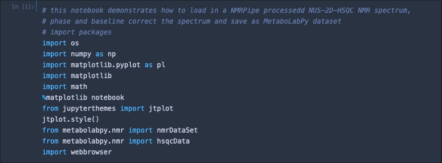
The first cell in this notebook loads necessary modules from installed packages. The second cell then downloads the sample dataset via an installed web browser.

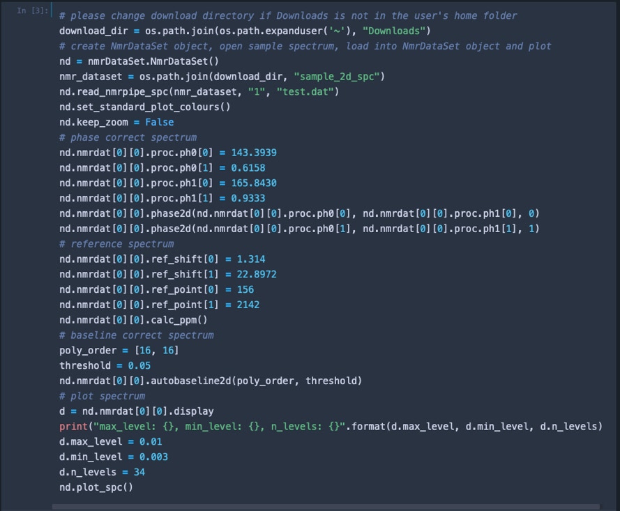
The downloaded dataset is then loaded into a MetaboLabPy nmrDataSet object, phase correction values for zero and first order phase correction are set for both dimensions, the spectrum is phase corrected, referenced and baseline corrected. Then plot parameters are set to ensure that the 2D plot does not render too much noise.

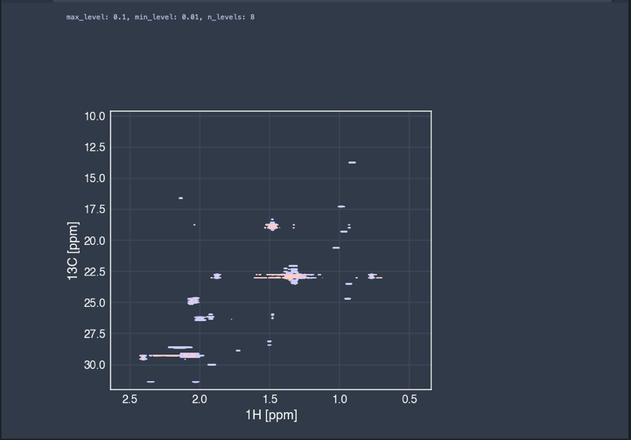
At the end, the resulting spectrum is plotted.

The spectrum is then saved as a MetaboLabPy data file.
