MetaboLabPy
Stable Isotope Tracing Analysis
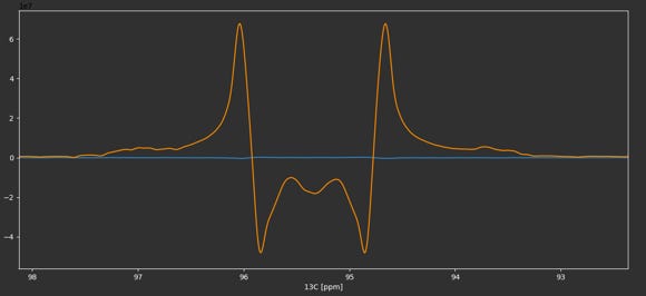
Sample data for this tutorial can be downloaded here. The NMR data with a highly resolved 2D-1H,13C HSQC NMR experiment is stored in experiment 2. We read in the NMRPipe processed 2D-NMR spectrum by clicking on Open NMRPipe or by using the keyboard shortcut Ctrl + n (⌘ + n on macOS). We phase correct, baseline correct and reference the spectrum to the methyl group resonance of lactate as described in Basic 2D-NMR Data Processing. Because of the high resolution in the 13C and because the pulse sequence used echo/anti-echo for quadrature detection, the signals in the 13C dimension show up as multiplets with dispersive line shape components due to the non-zero 13C-13C J coupling evolution in the first increment. We can use this line shape property to help with phase correction by ensuring that the minima of the line shape are at the same level (see below).
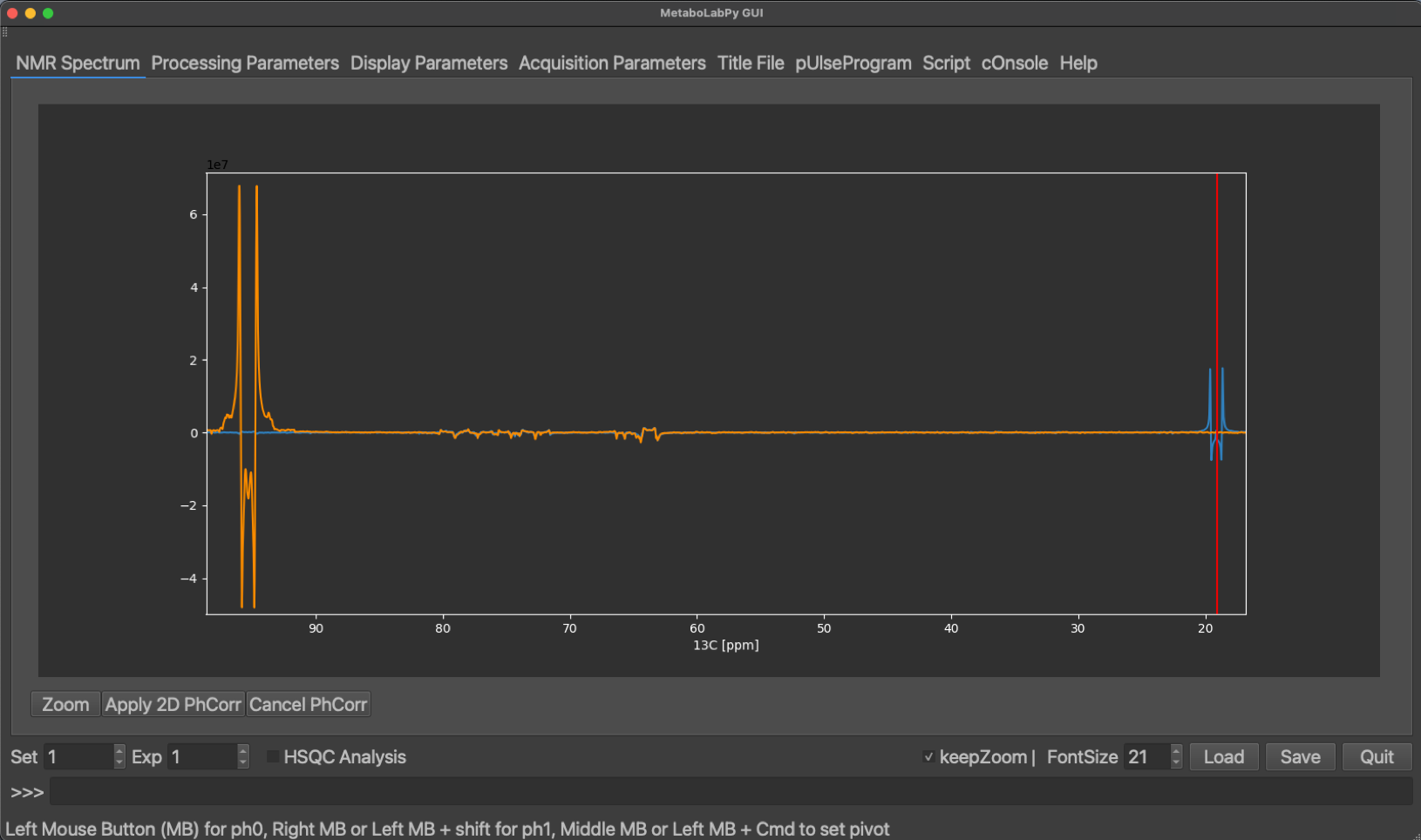
Before phase correction
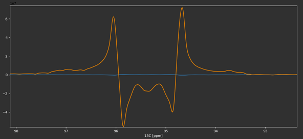
After phase correction
The phased, baseline corrected and referenced spectrum should look like the example below, where also the methyl group resonance of lactate is indicated.
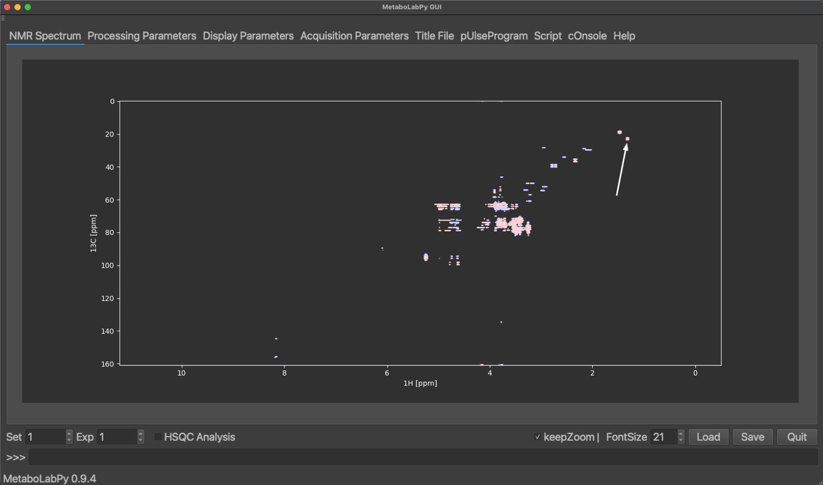
L-Lactic Acid
Tracing analysis by NMR spectroscopy is a two-step process. We have to describe the NMR multiplet composition (multiplet analysis) and then combine this information with per carbon 13C percentages or gas chromatography-mass spectrometry (GC-MS) data, which is described here.
When the software detects that a 2D-1H,13C HSQC NMR spectrum has been read in, the HSQC Analysis checkbox appears on the main window. Once this is checked, an additional tab appears which allows to perform multiplet analysis. In order to be able to perform multiplet analysis, pygamma (pip install pygamma) needs to be installed.
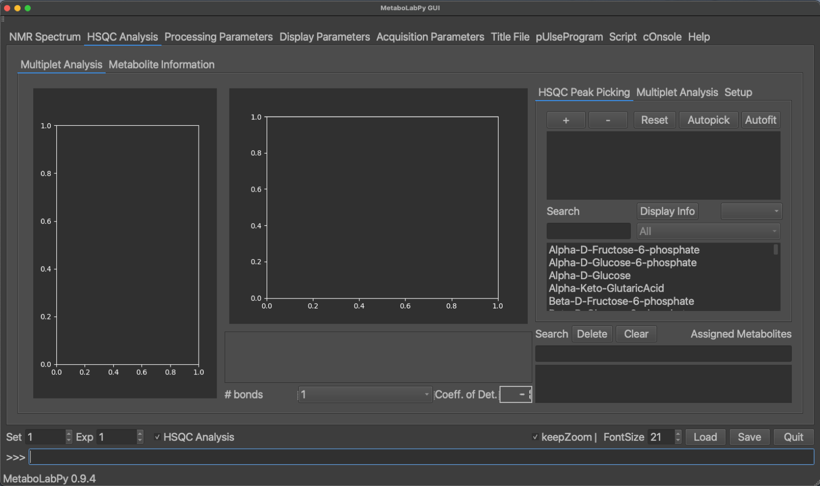
Chemical Structure
2D-Multiplet
1D-Multiplet
Metabolites
Assigned Metabolites
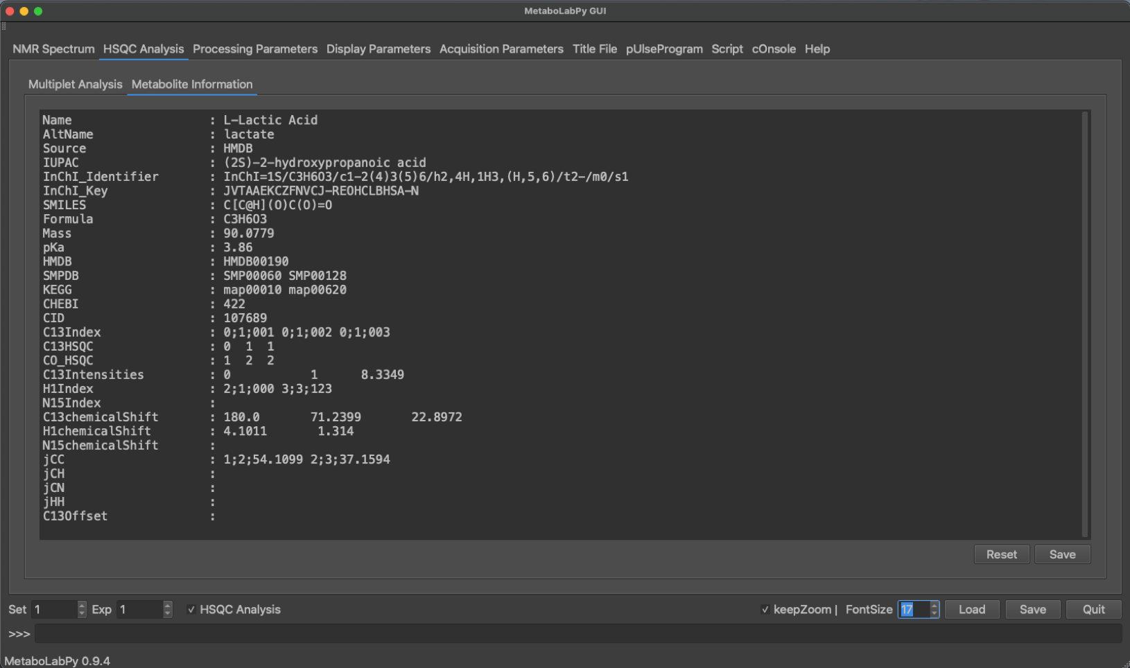
The HSQC Analysis tab has several GUI elements to facilitate multiplet analysis. Both the 2D-multiplet as well as a 1D-trace are being displayed. Once a metabolite has been selected a series of buttons, depending on the number of NMR signals for the selected metabolite, appear in the lower area of the middle of the tab. The chemical structure is displayed for each selected metabolite, and so are web links to HMDB and SMPDB. Once a metabolite is selected, Metabolite Information is filled in as well as demonstrated below.
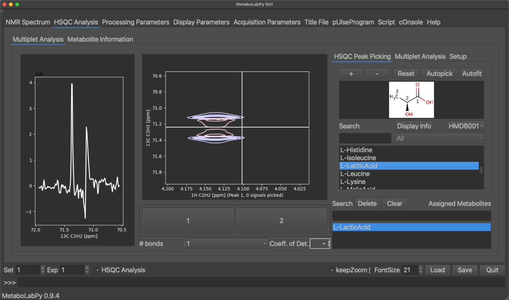
The peak display can be switched between the different metabolite signals using the buttons at the bottom of the tab. Peaks can be picked by clicking + (top right) or removed by clicking - and then selecting the desired peak. Alternatively an automatic peak picking algorithm (Ferrante et al.) can be employed by clicking Autopick. While only the currently selected peak is displayed, all peaks of the metabolite are picked using the automatic algorithm. A multiplet analysis can then be carried out by clicking on the Multiplet Analysis tab and then clicking on Fit. Alternativelyall peaks of the metabolite can be fitted automatically by clicking on Autofit in the HSQC Peak Picking tab. Once the line shape simulation is finished, the simulated trace through the 2D signal is displayed in yellow in the 1D-multiplet window. A confidence value (coefficient of Determination) is calculated indicating the quality of signal analysis. The display of this coefficient is colour coded (good, borderline, unreliable).
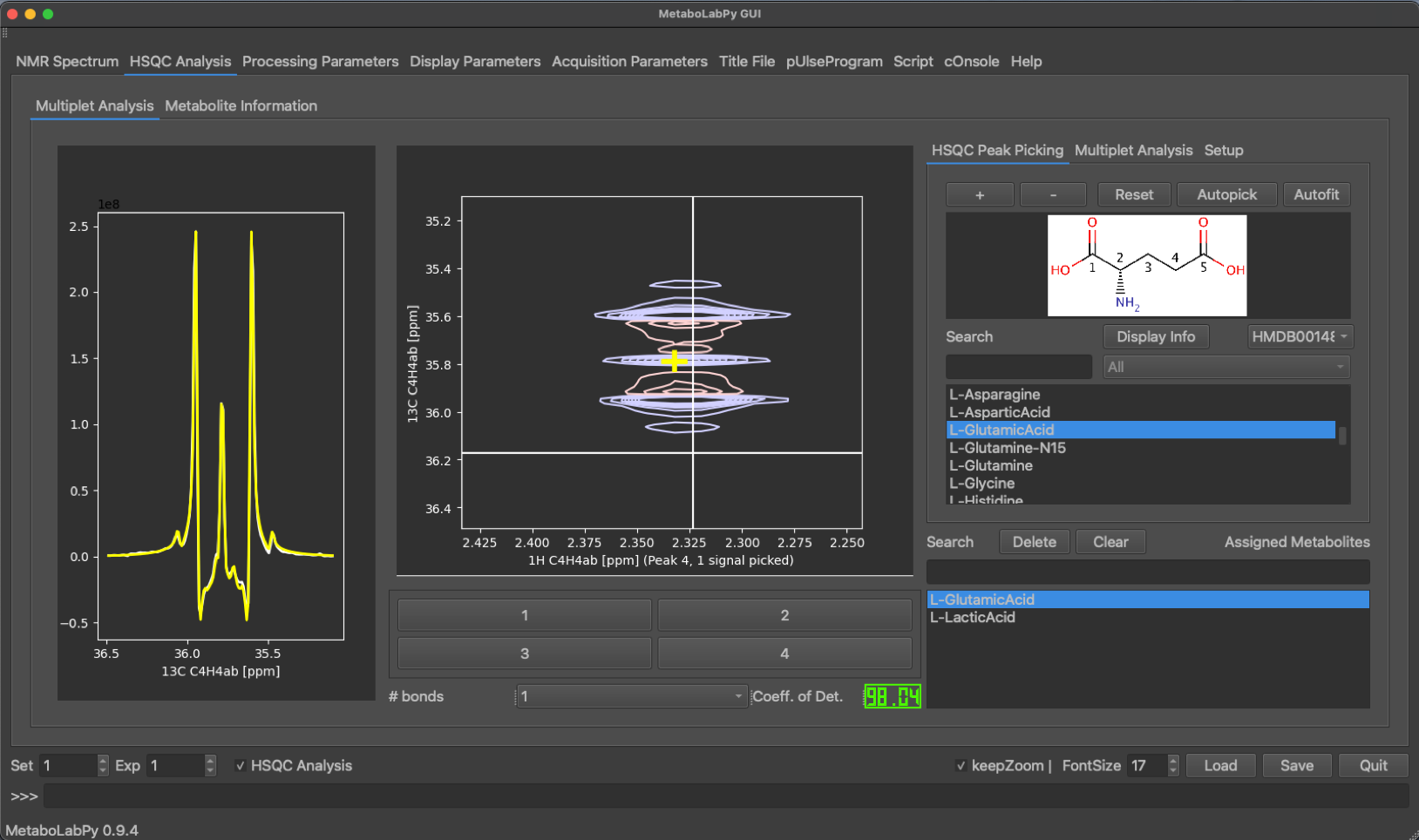
This analysis is then repeated for all metabolites of interest in all loaded HSQC experiments. The data can then be exported into an Excel spreadsheet for isotopomer analysis.
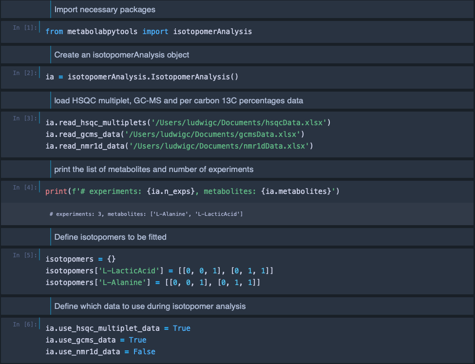
Isotopomer analysis is implemented within the metabolabpytools package and can most comfortably be carried out inside a jupyter notebook interface.
Please note: In order to be able to run jupyter notebooks, you must have the following to packages installed
- jupyter
- jupyterthemes
These packages can be installed with the command pip install jupyter jupyterthemes in an Anaconda powershelgl prompt or in a macOS Terminal, after the metabolabpy environment has been activated. For convenience, a zip archive with an example notebook (read_isotopomer_data.ipynb) as well as example spreadsheets for multiplet data, GC-MS data and per carbon 13C percentages can be downloaded here.
This is an example of a HSQC multiplet data spreadsheet:

Each metabolite is saved as its own worksheet, with all experiments for a single metabolite being contained in a single worksheet. The same is true for GC-MS and per carbon 13C percentages spreadsheets as demonstrated below.
GC-MS data spreadsheet:

Per carbon 13C percentages spreadsheet:

the data from these spreadsheets is then loaded into the jupyter notebook. Please note: Although we are loading in all three possible data sources, isotopomer analysis should be possible with a subset of these and we are only going to use multiplet and GC-MS data in the notebook to perform the isotopomer analysis.
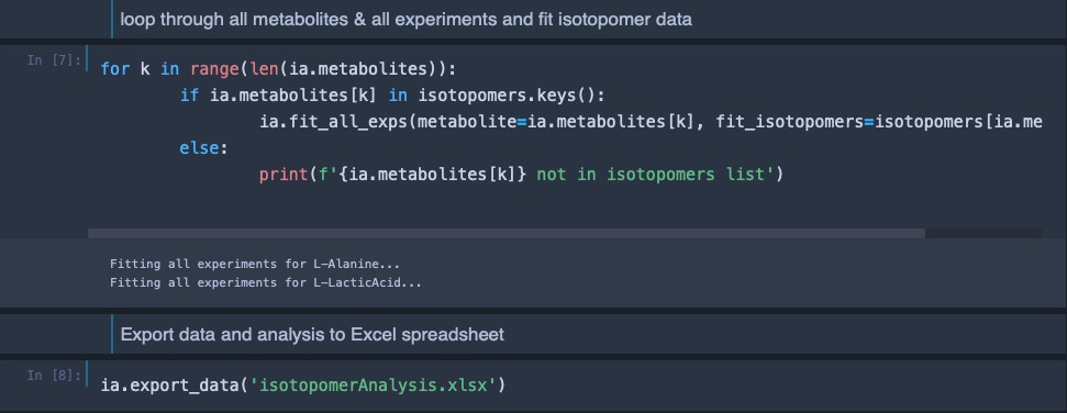
The final Excel spreadsheet with the results of the isotopomer analysis looks like this:
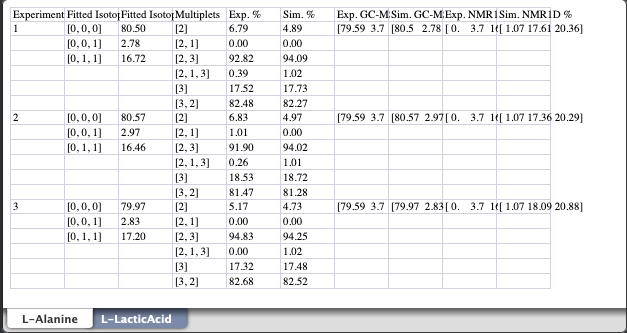
Despite per carbon 13C percentages were not used in the analysis, they are included as part of the simulated data.